FactorForge: I Built a Full Quant Research Pipeline — Here's What I Learned

What it is

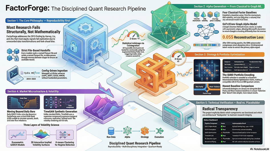
FactorForge is a seven-module quantitative research pipeline in Python. It takes raw daily stock prices and runs them through a disciplined sequence of stages: classical factor engineering, a graph neural network for alpha prediction, statistical arbitrage via cointegration, portfolio optimization with a quantum-ready encoding, GARCH volatility modeling, limit-order-book simulation using a generative AI model, and derivatives pricing with Greeks analytics.

The current implementation covers four stocks — Apple, Microsoft, Google, Amazon — across seven years of daily data from 2018 to 2025. Small by design. The goal was to build the architecture correctly before scaling it. Every module writes a named output file. Every downstream stage reads that file. Nothing passes through memory from one stage to the next. And every run is logged to MLflow with its parameters and artifact paths, so there is always a record of what produced what.

---

The pipeline problem nobody talks about

In 2016, Harvey, Liu and Zhu published a paper estimating that most equity return signals published in academic research fail when someone else tries to replicate them on new data. The failure is almost never mathematical. It is structural. Data transformations that were never written down. Factors computed with look-ahead information — tomorrow's data used to predict today's prices. Results that changed when the notebook was rerun and nobody noticed.

This is not a niche academic problem. It is the most common failure mode in quantitative research. And most learning resources teach the models without teaching the discipline.

FactorForge is built to enforce that discipline structurally. Every stage reads a Parquet file and writes a Parquet file. The backtest reads the alpha predictions file — it does not call the GNN. The portfolio optimizer reads the alpha file and the covariance file — it does not know how the alpha was produced. If you retrain the GNN with different settings, the backtest will produce a different Sharpe, because those are different experiments and they should produce different numbers. The separation is not engineering overhead. It is the reproducibility guarantee.

---

Stage by stage

Classical factors first

The pipeline starts deliberately unimpressively. Four numbers per stock per day: twelve-month price momentum, three-month momentum, sixty-day realized volatility, and a size proxy computed from log of price times volume.

These are the same factor families Fama and French documented in 1993. They have been replicated, extended, and debated for thirty years. They are baselines, not edge. The first rule of quantitative research is: understand what the simple methods produce before adding complexity. If your model cannot beat four classical factors, it has not learned anything the market does not already know.

A graph neural network for alpha

The novel piece of the pipeline is the alpha model. Instead of treating each stock independently, it builds a graph — four nodes, one per stock, with edges encoding relationships between them — and trains a GATv2Conv graph attention network autoencoder on that structure.

The architecture has two graph attention layers. The first expands to 128 dimensions using four attention heads. The second compresses down to a 16-dimensional latent vector. A linear decoder then tries to reconstruct the original return sequences from that compressed code. The training objective is reconstruction loss — the model is forced to find the most informative compression of each stock's return dynamics given its relationship to the others.

The alpha signal comes from the first dimension of that 16-dimensional latent vector.

The choice of GATv2Conv over standard GAT matters technically. The original Graph Attention Network computed attention weights from each node's own features independently, making attention effectively symmetric and static. GATv2 fixes this by applying the scoring function to the joint representation of both nodes — source and target combined — enabling the model to learn asymmetric relationships. In financial terms: how Microsoft's return history informs the encoding of Google's behavior can differ from the reverse. After 200 training epochs, reconstruction loss settles near 0.055.

Statistical arbitrage via cointegration

With alpha scores produced, the pipeline branches. The statistical arbitrage module tests all six possible stock pairs for cointegration — the formal property that two price series, while each wandering individually, have a spread that tends to return to a stable mean.

The test is the Augmented Dickey-Fuller test on the OLS regression residual. If the p-value is below 5%, the spread is stationary and the pair is accepted. The spread is then normalized into a z-score. Go long when the z-score falls below minus two — the spread has widened below its mean. Go short when it rises above plus two. Go flat when it returns toward zero.

This is the pairs trading framework formalized by Gatev, Goetzmann and Rouwenhorst in 2006. It is not a novel idea. Its value here is as a rigorous, theory-grounded baseline for measuring whether the graph structure produces genuine pair-selection insight.

Portfolio construction and the QUBO matrix

Three portfolio strategies run on the same alpha signal and covariance matrix, side by side.

Mean-variance takes the covariance matrix, inverts it via Moore-Penrose pseudo-inverse, and multiplies by the alpha vector to produce weights that maximize expected return per unit of risk. Risk parity gives equal weight to every stock — it ignores the covariance matrix entirely and is surprisingly robust because it sidesteps estimation error, which is the main practical failure mode of mean-variance. The QAOA-inspired strategy averages the two.

The more important output is the QUBO matrix. QUBO stands for Quadratic Unconstrained Binary Optimization — the standard encoding format for quantum portfolio problems. FactorForge constructs it from three terms: the covariance matrix as a risk penalty weighted at 0.2, the GNN alpha vector as a return incentive on the diagonal, and the graph adjacency matrix as a diversification penalty weighted at 0.1.

That formulation is economically coherent and mathematically complete. A D-Wave quantum annealer, an IBM QAOA circuit, or a classical simulated annealer can take it directly and solve for binary portfolio weights. The quantum solver is currently a classical blend used as a placeholder. The encoding is real.

Volatility modeling

Volatility is covered at three levels.

GARCH and EGARCH model volatility clustering — the well-documented tendency for large market moves to arrive in groups — with EGARCH adding the leverage effect: negative return shocks increase future volatility more than positive ones of equal magnitude.

Implied volatility surfaces render the full strike-and-maturity structure of market-implied volatility in 3D, capturing the vol smile and term structure that flat-vol Black-Scholes misses and that most derivatives pricing research is concerned with explaining.

K-means clustering on rolling realized volatility identifies high, transition, and low volatility regimes over the full seven-year window. And a diagnostics panel compares the autocorrelation structure and fat-tail properties of real volatility against TimeGAN-generated synthetic sequences — checking whether the generative model preserved the stylized facts that practitioners rely on.

TimeGAN and the order book

Daily prices hide everything that happens inside the trading day. The LOB module addresses this gap.

A baseline synthetic limit-order book is generated with Brownian-motion midprice, Gaussian spread, and random order flow imbalance. But the more interesting component is the TimeGAN model trained on real LOB sequences. Standard generative adversarial networks fail on time-series data because they learn marginal distributions — what each timestep looks like — without preserving temporal structure — how sequences evolve. TimeGAN addresses this with a supervisor component that enforces temporal coherence in the latent space during training. The result is synthetic order-book paths that preserve spread clustering, order flow imbalance autocorrelation, depth dynamics, and fat-tail midprice return distributions.

The practical value is a realistic synthetic data source for testing execution algorithms without requiring proprietary real-time feeds.

Derivatives pricing

The derivatives module prices options three ways — Black-Scholes analytically, Crank-Nicolson PDE solver numerically, and Monte Carlo with variance reduction — then validates each method against the analytical benchmark for vanilla cases. Delta, gamma, and vega are computed and rendered as 3D surfaces over strike and maturity grids. Local volatility calibration using Dupire's formula backs out the instantaneous volatility function consistent with observed market prices, which is the standard approach for pricing exotic derivatives consistently with vanilla market quotes.

---

What I'd tell someone building something similar

Name every output. The single most important architectural decision was requiring every stage to write a Parquet file with a specific name, and every downstream stage to read that file. This one constraint prevents look-ahead contamination, makes the pipeline auditable, and forces you to think about what the actual output of each stage is before you start writing it.

Run baselines in parallel, always. Risk parity is computed alongside mean-variance and the QAOA blend on every run. On some periods it wins. When it does, that result is visible. Research that only shows you the periods where the advanced method won is not research — it is selection.

Be precise about what is and is not implemented. The QAOA portfolio is a classical blend and a solver hookpoint. The QUBO matrix is real. The quantum computation is not wired in. The RL execution agent has an environment but placeholder training logs. All of this is labeled explicitly in the documentation. That precision is not modesty — it is the practice of knowing what you actually know versus what you have prepared infrastructure for.

The connections between modules are the hardest and most valuable part. GARCH volatility forecasts feeding derivatives pricing. GNN alpha feeding both portfolio construction and the QUBO encoding. TimeGAN LOB sequences feeding execution simulation. Understanding how these disciplines connect in a production pipeline is rarer than knowing any one of them individually.

---

Real-World Applications

GATv2Conv Alpha Model

• Equity hedge funds use graph-structured models to capture sector contagion and cross-asset spillover that linear factor models miss — GNN-derived latent factors sit alongside Barra-style risk factors for alpha decomposition

Statistical Arbitrage

• Stat-arb desks run cointegration-based pairs books across thousands of equities; the same z-score framework applies directly to ETF-vs-basket arbitrage and fixed income relative value (on-the-run vs off-the-run Treasuries)

QUBO / Quantum Portfolio Encoding

• D-Wave and IBM benchmark quantum annealers on real portfolio selection using this exact QUBO input format; classical solvers already use it in production for cardinality-constrained and sector-capped allocation problems convex optimizers cannot handle natively

Volatility Modeling

• Options market-makers use GARCH forecasts for hedge frequency decisions; risk teams use EGARCH for VaR/ES; the regime clustering module maps directly to risk-on/risk-off position sizing rules at systematic macro funds

TimeGAN / LOB Simulation

• Execution desks use synthetic order-book environments to backtest TWAP, VWAP, and implementation shortfall algorithms before live deployment; regulators use synthetic microstructure data to stress-test market structure without waiting for real crises

Derivatives Pricing

• Structured products desks run Dupire local vol calibration daily to reprice exotic books against vanilla market quotes; Monte Carlo with variance reduction is the production standard for path-dependent payoffs where closed-form solutions do not exist

Pipeline Discipline

• Systematic funds run this exact pattern — config-driven experiments, versioned artifacts, tracked runs — as the foundation of live research infrastructure; the Parquet artifact chain is one scheduler swap away from a production data pipeline